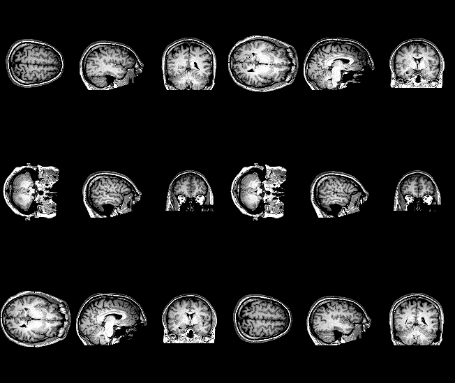
Introduction

While major strides have been made in deep generative modeling, including significant advances in natural language, image, and video generation, there remains a disconnect between these technical advances and practical applications, especially for social good. A critical application area for deep learning is healthcare, where high-stakes decision-making occurs daily and learning algorithms can directly improve lives. In my own research, and in the broader machine learning for healthcare community, the focus has largely been on discriminative and prescriptive modeling. These approaches are directly motivated by the problems encountered in health applications, such as predicting the risk of developing a disease, predicting whether a scan includes a tumor, or prescribing the best treatment to maximize patient outcomes. Recently, language-based generative models have gained traction as a practically useful tool in healthcare tasks, assisting with summarization, feature extraction, and even structured prediction [Agarwal et al. 2022, Moor et al. 2023]. The flexibility of natural language, along with the impressive zero-shot and in-context learning ability of these models, allows them to perform a large variety of useful tasks. However, the motivation for image-based generative modeling in health applications is less clear.

How might we use generated images to improve healthcare operations and outcomes? Image data is ubiquitous in healthcare, from X-Rays to MRIs and CT scans, to histopathology (microsopic imaging of tissue and cells). However, unlike other applications, image data in healthcare is highly specific to each patient, and “creativity” in the image output would be viewed as a detriment, not an opportunity. Therefore, image-based generative models for healthcare must provide either significant discriminative ability or be carefully conditioned on existing patient data. That is, there are two primary avenues for image-based generative models to improve healthcare:

1. Image Reconstruction. Due to how expensive and time-consuming certain imaging techniques are, such as MRIs and CT scans, it has become important to downsample or sparsify the measurements taken for these images. As a result, the inverse problem of reconstructing the true image from the partial measurements is ill-posed, making reconstruction a challenging task. This is naturally a conditional image generation problem.

2. Public Synthetic Dataset Generation. An acute problem in ML for healthcare is the accessibility and availability of patient data. Patient data is traditionally kept on-premise within hospital networks, necessitating all research be conducted with the compute resources available within those individual networks. In practice, this dramatically slows the rate of research and development, as researchers wrestle with high latency, antiquated hardware, small datasets, and limited compute resources. There is therefore an exciting and promising direction for generative modeling to resolve this problem by allowing us to generate synthetic data, which could potentially be used outside of the hospital networks.

Solving Inverse Problems with Generative Models

At a high-level, we can pose the image reconstruction problem for medical images as follows: let \(y \in \mathbb{R}^m\) be some low-dimensional representation of a raw input image $x \in \mathbb{R}^n$, generated by the linear transformation $y = Ax + \epsilon$ where $A \in \mathbb{R}^{m \times n}$ and $\epsilon \in \mathbb{R}^m$ is a noise vector. That is, $y$ is a noisy projection of the raw input image $x$ onto a lower-dimensional space. Our goal, ultimately, is to collect only the lower-dimensional measurements $y$ and solve the inverse problem to recover the most likely full image $x$ corresponding to $y$. This can save patient time, improve patient safety, and reduce hospital costs. For a given transformation $T: x \rightarrow Ax + \epsilon$, this inverse problem can be treated as a supervised learning problem, for which we have pairs $\{(x_i, y_i)\}_{i=1}^N$ of images and their corresponding projections (Wei et al. 2022). However, in practice, this transformation can vary significantly, even for the same type of image. For example, one hospital might be taking $m=10$ measurements, while another hospital might be taking $m=25$ measurements. The transformation matrix $A$ applied may also be different, separate from the number of measurements. This would require generating pairs of measurements and raw image data for each physical machine creating this data.

Rather than thinking of this as a supervised learning problem, Song et al. (2022) propose addressing this problem with unconditional image generation. The key, as we will soon discuss, is to guide the image generation at inference time by nudging the generated image toward satisfying the condition $y = Ax$, where $y$ is the actual measurements, and $x$ is the generated image. The first step is training an unconditional score model $s_{\theta^*}(x, t)$ on a dataset of full images (e.g. CT scans or MRIs). At inference, we expect to only have some measurements $y$, for which we can generate a conditional stochastic process $\{y_t : y\}_{t \in [0,1]}$ by using the linear relationship,

and, noting that $x_t \sim \mathcal{N}(\alpha(t)x_0, \beta(t)^2I)$, we can derive the relation

where $z \sim \mathcal{N}(0,I)$ and $\alpha(t), \beta(t)$ are noise schedules. Therefore, $y_t$ is an interpolation between the true measurements $y$ and noise $z$ that has been projected to the same space as $y$ through the transformation matrix $A$.

From this point, the traditional iterative sampling process would sample timesteps $\{0=t_1 < t_2 < \dots < t_n=1\}$ and produce observations

where $h$ could be given by the Euler-Maruyama sampler,

In their work, Song et al. (2022) propose an additional step in this denoising process that corrects for the measurement process,

where, critically, the function $k$ solves a proximal optimization step that aims to minimize the distance between $x_{t_i}$ and $x_{t_i}’$ while also minimizing the distance between $x_{t_i}’$ and the hyperplane $\{x \in \mathbb{R}^n : Ax = y_{t_i}\}$. That is, $x_{t_i}’$ should be a projection of $x_{t_i}$ onto the feasible set $\{x \in \mathbb{R}^n : Ax = y_{t_i}\}$. With the hyperparameter $\lambda \in [0,1]$, the optimization problem becomes

where $\lambda$ controls the relative importance of the two objectives. Notice when $\lambda = 1$, we guarantee that $x_{t_i}’$ satisfies $Ax_{t_i}’ = y_{t_i}$. In practice, the authors use Bayesian optimization to tune this hyperparameter empirically. Using a decomposition for the transform matrix $A$ (which only assumes $A$ is full rank), the authors are able to derive a closed form solution for $k$, such that this step is both exact and efficient. A visualization of this process is given below.

Guided generation of samples from an unconditional score model from Song et al. (2022)

At this point in time, this approach represents the state of the art in solving such inverse problems, even matching or outperforming supervised learning approaches while providing significant flexibility. In the figure below, we can see that this approach yields both the highest PSNR and SSIM scores for a dataset of CT scans. Looking closely at the zoomed in segments, it is clear that their approach captures significant detail that some of the other results lack. These finer details are crucial in real applications, when, for example, a radiologist is reviewing a scan, trying to identify subtle changes in the patient’s physiology. In my opinion, this idea of guiding unconditional genertive models at inference is extremely promising for a variety of applications, but especially in healthcare, where labeled data is less readily available and conditions change across different hospital systems.

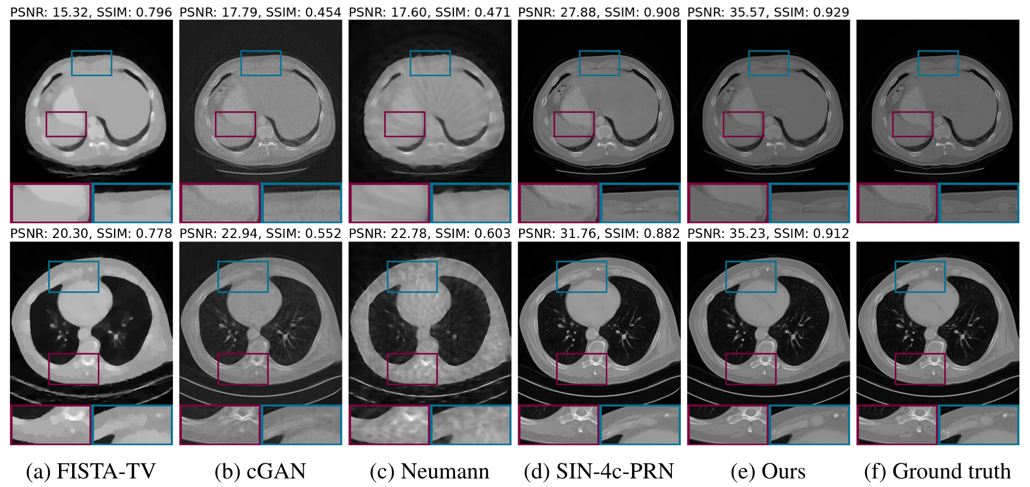Results from Song et al. (2022) applied to CT dataset.

Coming from a background in Operations Research, the proximal optimization step that guides the image generation is particularly interesting. While the authors do not provide this ablation study, I would be curious to see how the generated images change qualitatively for varying values of $\lambda$. It is possible that when $\lambda=1$, the resulting image $x_{t_i}’$ looks somewhat unrealistic. Recall that when $\lambda=1$, the generated image $x_{t_i}’$ is a projection of $x_{t_i}$ onto the hyperplane $\{x \in \mathbb{R}^n : Ax = y_{t_i}\}$. While this point may be the closest in space to $x_{t_i}$ that satifies the measurement process, it may be that this point contains unrealistic artifacts. Instead, an alternative approach could be to follow a path from $x_{t_i}$ to the feasible hyperplane that maximizes the likelihood of $x_{t_i}’$. Given that we don’t typically have access to the marginal distribution $p_t(x_t)$, we could instead find a path along which the score function is maximized. More formally, suppose we have a current sample $x_t$ with a corresponding measurement $y_t$. Then maximizing the score along some path $\gamma$ from $x_t$ to the hyperplane $Au = y_t$ at some point $x_t’$ gives us

However, we don’t typically have access to $p(x_t’)$, but we do have access to $s_{\theta^*}(x_{t}, t) \approx \nabla_{x_t}\log(p(x_t))$, which we can use to recover a path that increases $p(x_t’)$.

While likely less efficient than the proximal update step, which has a closed-form solution, there are multiple ways that this formulation could be approximately solved. For example, discretizing the space between $x_{t_i}$ and the feasible hyperplane, one could evaluate the score function at each grid point and then solve a shortest path problem to find a path that maximizes the total score. Alternatively, one could follow an iterative approach, where at each step the score function $s_t = s_{\theta^*}(x_{t_i}, t_i)$ is evaluated, the resulting gradient vector is filtered such that only the components in the direction of the feasible hyperplane are kept, and $x_{t_i}$ is updated in the direction of this vector. That is, suppose $\mathbf{n}_t$ is the normal vector to the hyperplane $Au = y_t$, then we would do

Where $\eta$ is our step-size, and $s_{proj}(x_t, t)$ selects the components of $s_{\theta^*}(x_{t}, t)$ that are in the direction of the feasible hyperplane. In the case $||s_{proj}(x_t, t)|| \approx 0$, we could default to the proximal step. This process could be repeated multiple times until $x_t’$ approximately satisfies the measurment constraints. Crucially, such approaches could eliminate the need for the sensitive hyperparameter $\lambda$, and may produce higher quality, more realistic results. I provide a visual of this idea below. In the visual, I propose that the point $x_t’’$ is better than $x_t’$ as it satisfies the measurement conditions while following the gradient of the log likelihood. The faint blue lines represent the vector field of the gradient of the log-likelihood.

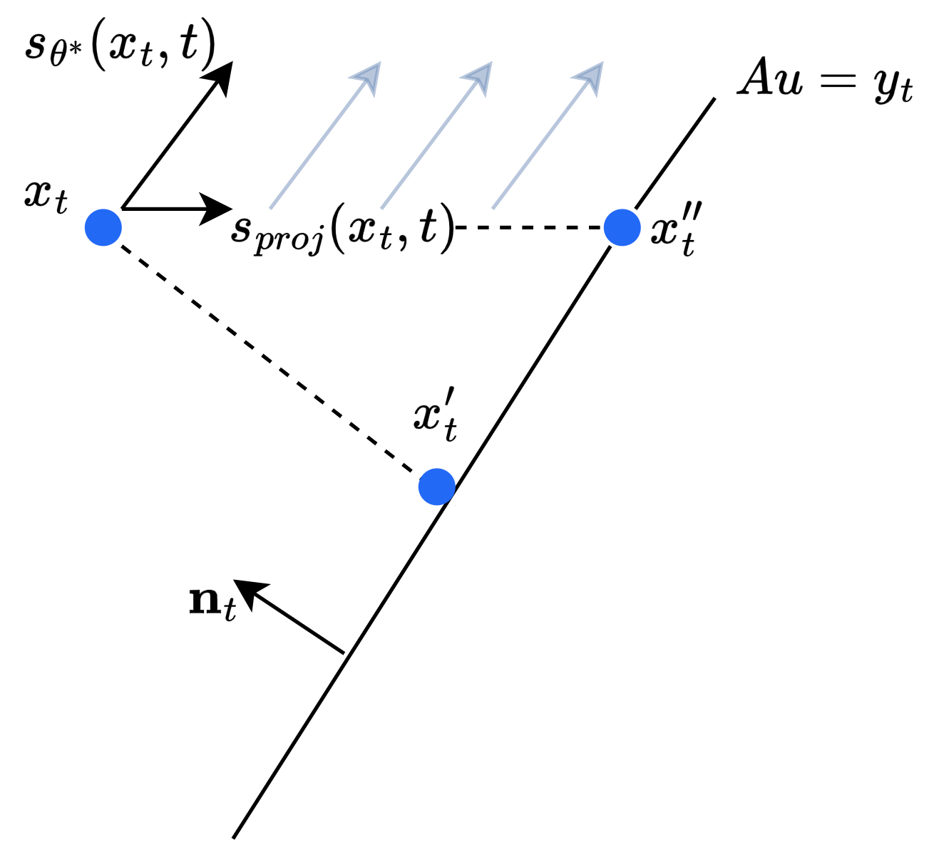An illustration of the energy-minimizing approach I propose for finding samples that satisfy given constraints.

Extension to Consistency Models

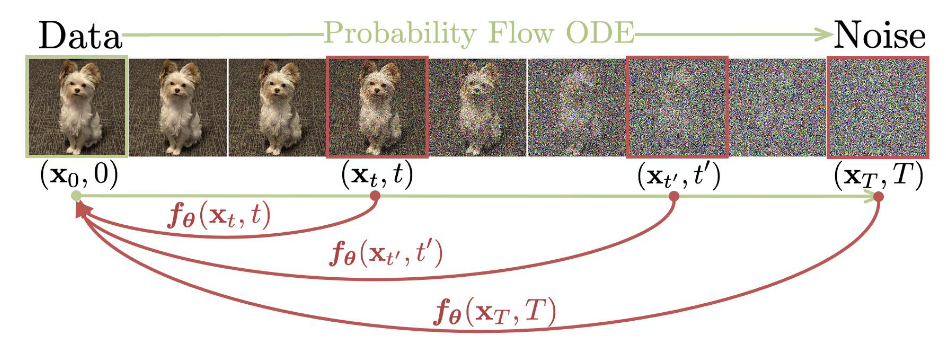A consistency model learns to map any point on the ODE trajectory to its origin. From Song et al. 2023

One drawback of the score matching diffusion models described in the previous section is that inference is often quite slow due to the many iterations involved in the generation process. Further modifications to the generation process, such as the additional update steps proposed, and especially the steps I suggested as future work, would only slow down this process further. The recently developed Consistency Models (Song et al. 2023) offer an alternative few-step diffusion approach that achieves impressive performance using a fraction of iterations required for traditional diffusion models. While a sufficient introduction to Consistency Models is outside the scope of this blog, at a high level these models learn a denoising function $f: \mathcal{X} \times [0,1] \rightarrow \mathcal{X}$ that is self-consistent such that $f(x_t, t) = f(x_{t’}, t’)$ for any pairs $(x_t, t)$ and $(x_{t’}, t’)$. Imposing the boundary condition $f(x_0, 0) = x_0$, the model then learns to map any noised input to the original pixel space in a single step. Sampling can be done in an iterative, multi-step process as well, where pure gaussian noise is denoised using the model, then some noise is added back and the model is used again to denoise the result. The impact of this iterative denoising seems to decay after four or five steps, but tends to yield better results than single-step generation.

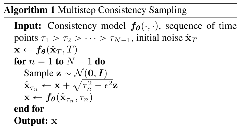The consistency model sampling algorithm from Song et al. 2023

Notice, however, that the process used to generate images at inference is quite similar, visually, to the guided process for generating images in the previous section. In fact, such a proximal optimization step can be easily incorporated into the Consistency Model framework. In their work, Song et al. (2023) describe such an approach as zero-shot image editing. The model itself would be trained as usual, to perform unconditional image generation. Then, at each step of the sampling process, prior to adding noise, we apply the proximal optimization step as defined in the previous section. This would achieve the same goal of guiding the generation process according to the measurements, but it would do so with only a few iterations.

To further motivate the idea I mentioned in the previous section, I trained my own unconditional consistency model on the MNIST dataset and tried guiding the sampling procedure following the correction approach proposed in Song et al. (2022). Specifically, the lower order representation I create is simply the bottom half of the original image. Therefore, the model must essentially complete the top half of the image (similar to how inpainting is done). I provide a visualization of some of the results below. While I experimented with the $\lambda$ hyperparameter, I found that for $\lambda < 0.98$, the generated samples completely ignored the measurement conditions. As an aside, in the Consistency model paper, the zero-shot editing algorihtm is actually almost equivalent to the proximal optimization step posed in Song et al. (2022), except that $\lambda = 1$ always. I suspect this is a property of consistency models and the way they denoise samples. It is likely that taking such a large step, from pure noise ($t=T$) to a realized sample ($t = 0$) imposes too much structure in the output, and the distance between the output and the measurement constraints is too large to be corrected. In the visualization below (with $\lambda = 1$), some of the completions look like real digits. However, notice how the last sample looks like a one stuck onto the bottom of a four or a nine. While the image satisfies the measurement constraints, I argue that snapping the samples to a low energy point that satisfies the constrain, rather than the closest point, might resolve this issue.

Selected output from consistency model with zero-shot editing for MNIST

Public Synthetic Dataset Generation

We now turn our attention to the other major area for generative image models in healthcare - creating useful, anonymized public synthetic datasets. These two terms, useful and anonymized, characterize the necessary conditions for such image generation in healthcare. More specifically, any such dataset must have:

• Discriminative Ability. The synthetic data should allow us to learn patterns that generalize to the true data distribution.
• Privacy. The generated data must not leak information from the original training data.

While there is an abundance of research papers applying the latest generative modeling techniques to clinical imaging data, very few address these two critical concerns. Perhaps the most interesting recent work to tackle this problem is the paper “Differentially Private Diffusion Models Generate Useful Synthetic Images”, written by a group at Google DeepMind. The title is a bold claim, but the authors do indeed produce signficant performance improvements on downstream tasks over previous work. Importantly, they address both characterisitics in the context of diffusion models.

Differentially Private Diffusion Models

While there has been recent interest in content removal and privacy in the context of deep generative models, most of this work has been focused on removing specific concepts or training samples, often referred to as “unlearning” [Wang et al. 2024]. This isn’t quite what we need, since we want to ensure privacy for all patients in the training dataset. Instead, what we want to achieve is generally referred to as differential privacy. If we have two training datasets $D$ and $D’$ that differ by exactly one training sample, we say algorithm $A$ is $(\epsilon, \delta)$-differentially private if

where $S$ is the support of $A$. In english, this simply means that changing the training data by one data point (e.g. one patient) is unlikely to change the output of the algorithm, where $(\epsilon, \delta)$ determine how strict this privacy requirment is. In the context of generative vision models, where the output of $A$ is in the original pixel space, differential privacy implies that adding or removing a single image from the training data is unlikely to change the output distribution of the model. Critically, the probability that the model returns something close to the specific image in the training data that was added or removed should not change (by much).

To achieve differential privacy guarantees for deep learning models, the standard approach is to train the model using the aptly named differentially-private stochastic gradient descent (DP-SGD) [Song et al. 2013]. The intuition behind this approach is straightforward - differential privacy is guaranteed by clipping the gradients of the model weights and adding gaussian noise parameterized according to the $(\epsilon, \delta)$ privacy terms. Formally, the mini-batch gradient $\hat g$ is computed as

where $\zeta \sim \mathcal{N}(0, I)$, $C$ represents the max $l_2$-norm of the weight gradient and the deviation $\sigma$ is determined by the privacy parameters. While this approach achieves our desired privacy guarantees, noising the gradient at each batch step significantly slows model training and leads to worse performance on traditional classification tasks. Applying DP-SGD to diffusion models, as Ghalebikesabi et al. (2023) do in their work, using a traditional U-Net DDPM [Ho et al. 2020], this problem is compounded by the noise injected into the training of model during training. The authors address this point directly in their paper.

“Thus overall, it is currently not obvious how to efficiently and accurately train diffusion models with differential privacy.” - Ghalebikesabi et al. 2023

One partial solution to address this problem is to pretrain the diffusion model on a public dataset, such as ImageNet, without differential privacy. In experiments, Ghalebikesabi et al. 2023 finds this pretraining yields a significant improvement when fine-tuning on a different data distribution using DP-SGD. While pretraining and carefully adjusting the training hyperparemeters can lead to improved performance, there still remains a significant gap. In my opinion, this is a major open problem where a positive result, reducing or eliminating the compounding noise effect of training differentially private diffusion models, could have a significant impact on open-source, large scale research in data-sensitive domains such as healthcare. The problem is certainly non-trivial (and well beyond the scope of this blog), but there might be some way to combine the noising between the diffusion process and the parameter update step that can provably yield the same differential privacy guarantee. Perhaps part of the solution could be in the sampling step, since it is already a standard part of DDPM sampling to inject noise at each denoising step.

Regardless of future improvments with regard to privacy, Ghalebikesabi et al. 2023 demonstrate the practical use of the synthetic data generated by their differntially private diffusion modes for downstream tasks. Below, I’ve included some interesting empirical results from their paper. What they find is a strong positive correlation between the test accuracy on synthetic data and the test accuracy on real data. They also find that the hyperparameters yielding the best performance when training with the synthetic samples also produce the best results when training with the real data. These results suggest that the synthetic data does indeed have some utility, specifically, it demonstrates empirically that it can be used for hyperparameter tuning, which can be very time consuming and computationally expensive. Once the best hyperparameters are found, those results could be used to train a production model one time within a hospital network.

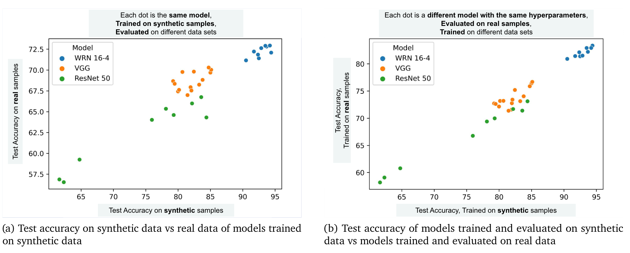Comparison of performance between synthetic and true data distributions from Ghalebikesabi et al. (2023)

While promising, one thing I noticed from their paper is that they only pretrain the diffusion models using ImageNet32 data. They do fine-tune and evaluate on a clinical image dataset, Camelyon17, a collection of 96 x 96 image patches of lymph node tissues, but they do not pretrain on a clinical dataset. For most medical imaging applications, there exists publicly available datasets already. The question is then, how much does the synthetic data further benefit our models during training? It would be very interesting and exciting if it is the case that the synthetic data, combined with existing relevant public datasets, further improves model performance on downstream tasks. For example, if I were to pretrain my diffusion model using the Camelyon17 dataset (which is, of course, public) and then fine-tune the model using some private lymph node imaging data from a hospital I’m collaborating with, would this model be more helpful for selecting hyperparameters than using the publicly available real data alone? I ask this question because I suspect I could generate results similar to the ones shown in the plot above by using public, real datasets alone. Therefore, while this work shows a positive result, that the synthetic data is useful for downstream tasks, it stops short of answering whether the synthetic data helps us more than the existing public datasets alone that we have already.

Scaling and Evaluation

Before I let you go, there’s one more set of challenges that I believe are critical to improving generative vision models for healthcare. The first is the issue of scale with regard to the image size. To capture the level of detail necessary for diagnostics, medical image data is often very high resolution, and often 3D. There’s also video data, both 2D and 3D. Scaling diffusion models, which are notorious for requiring many training steps to converge, to $256^3$-pixel volumetric MRI data is extremely challenging. Work such as Song et al (2022) circumvent this problem by taking 2D slices of 3D imaging datasets to train and evaluate their models. Other work, such as Ghalebikesabi et al. (2023), downsample the raw images before training. This, of course, limits the practicality of these models. For image reconstruction, it is likely that radiologists want multiple slices of the brain volume. Further, the slices should be consistent, such that stacking them yields a smooth, continous volume. Perhaps sampling from different slices during training could yield a model capable of generating whole brain volumes by generating each slice separately. We could go one step further and condition each slice on the previously generated slices. In any case, this remains an open problem, as scaling to 3D volumes directly does not seem currently feasible.

To demonstrate this point, I refer to recent work by Shibata et al. (2024), who attempt to create a differentially private 3D DDPM to generate $256^3$-pixel 3D structural brain MRIs. To decompose the problem, they train a separate model for each denoising step, corresponding to $T$ models, where $T$ is the total number of timesteps in the diffusion process. The authors posit that otherwise, a single neural network (of reasonable scale), could not handle the full complexity of modeling high-dimensional 3D gaussian noise. In the end, they set $T=200$, with 100m parameters per network, corresponding to 20B parameters in total. With eight dedicated A100 GPUS, the authors train their model for 4 epochs with a training dataset of only about 1000 samples. Therefore, with eight dedicated GPUs, it was still only feasible to train the model for about 4000 steps. Even with all this effort and time, the resulting model does not produce generated images that are satisfactory for clinicians. The output of the model was rated on a scale of 1-5 by a group of doctors for each region of the brain, grading the visibility of individual brain structures. The results of this study are shown below.

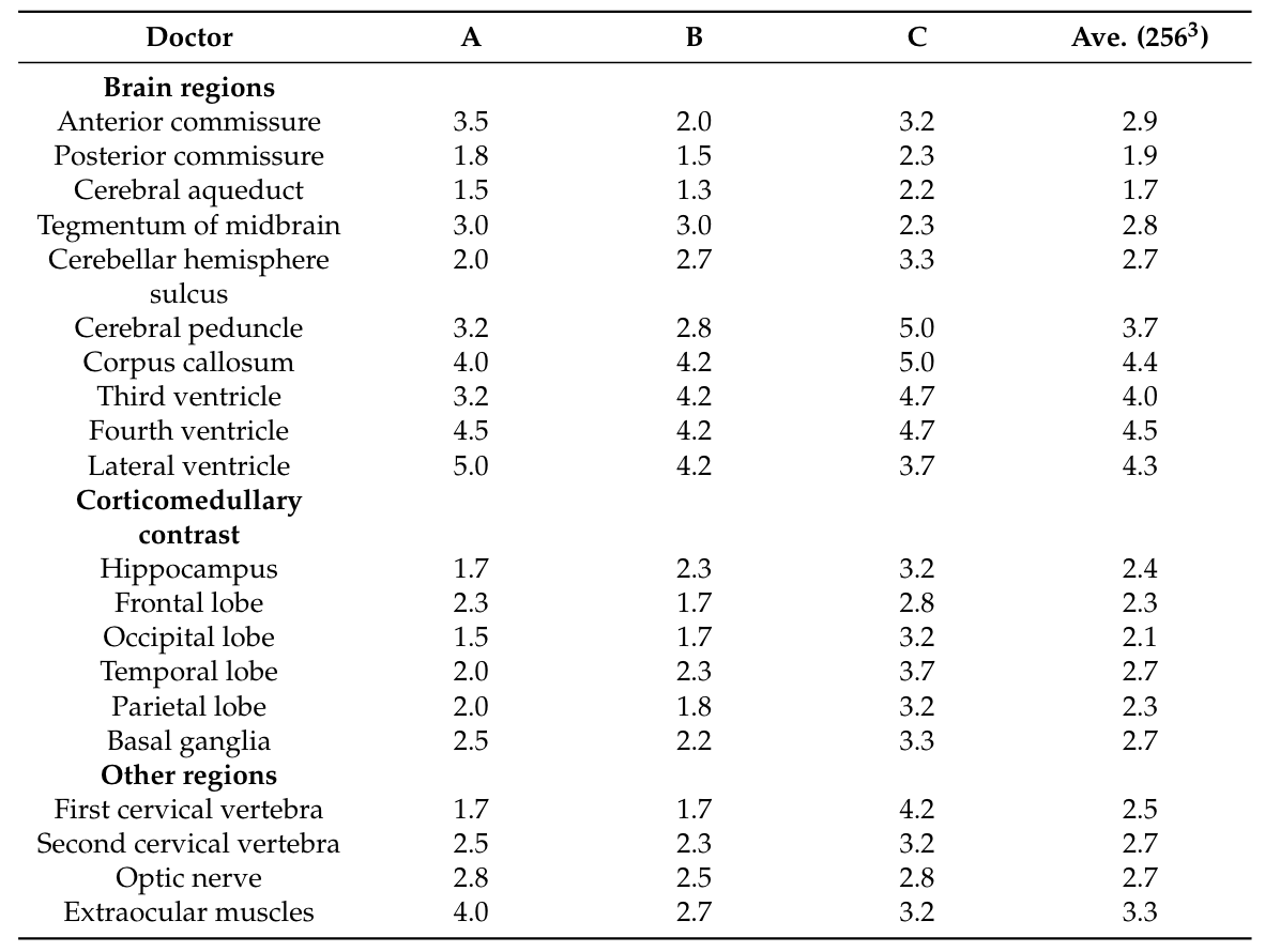Doctors’ grades of generated brain structures from Shibata et al. (2024). A score of 4 or greater indicates sufficient structure visbility.

It’s clear that the doctors were unable to identify most brain structures in the generated images. In fact, we can take a look at the generated brains ourselves and see that clearly, quite a bit of structure is lost from the original images. Many of the folds and much of the contrast is lost, with most regions of the brain becoming smooth blobs.

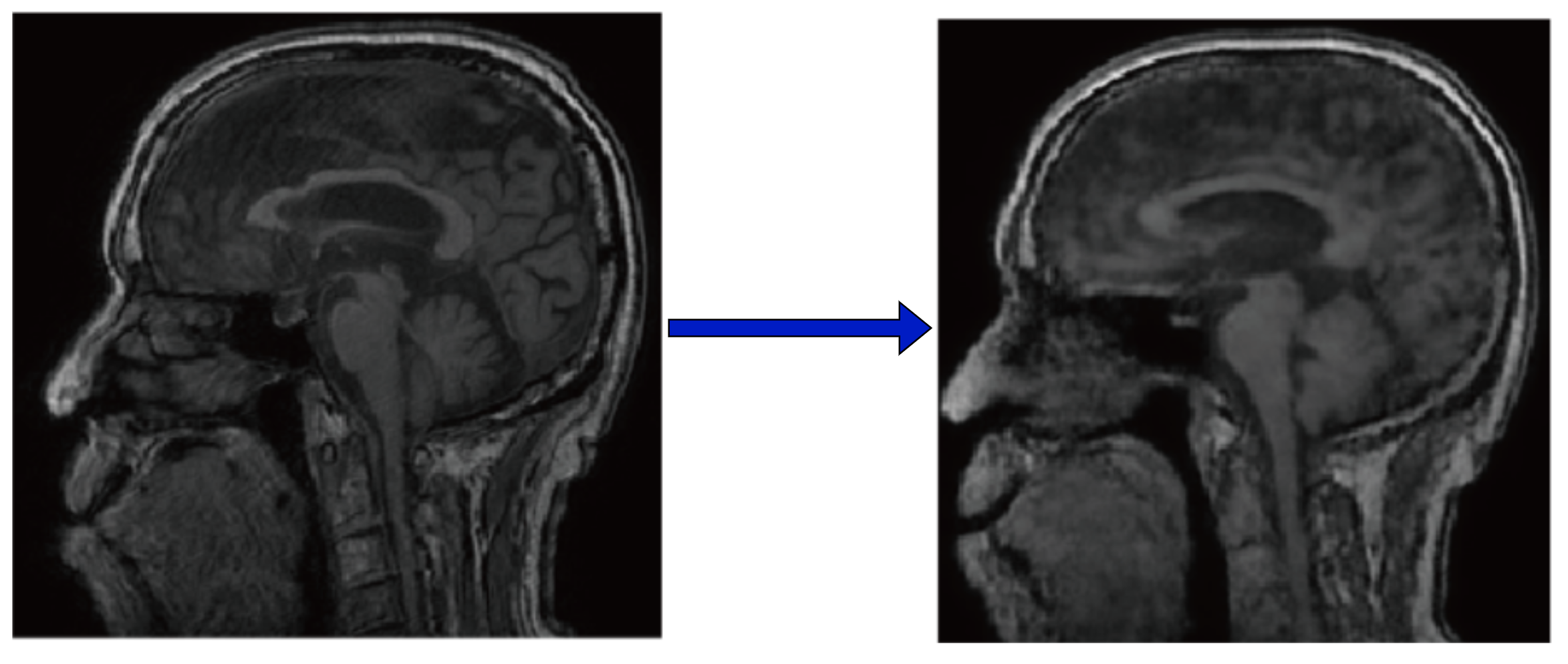Left: Original 2D slice of MRI. Right: Denoised output.

While future work will certainly improve upon this baseline, it is also impractical to expect doctors to manually grade the output of each new model created. This has led me to think more carefully about how we could evaluate the generated samples for brain MRIs, in addition to standard metrics like FID and PSNR. This gets to my second challenge, metrics and evaluation. One idea, similar to the FID score, would be to apply a brain segmentation model to the generated images, and evaluate the confidence and relative volume of the brain which the segmentation model labels as belonging to a specific brain region. More formally, a segmentation model takes the form $m: \mathcal{X} \rightarrow \mathbb{R}^{K+1}$ where $K$ represents the total number of defined brain segments, and the $K+1$-th class refers to unknown or non-brain matter. We could measure the output of this model, perhaps looking at the percent of pixels labeled as unknown, or the confidence of the model in the regions it labels as being a specific brain structure (e.g. the mean of the segmentation output). Such a metric connects directly to what radiologists care about, seeing clear brain structures, and are readily available.

Conclusion

If you’ve made it this far, I thank you. Overall, the opportunity for using generative vision models to improve healthcare operations is exciting, and there are more avenues to have a positive impact than I had previously thought. However, there are still major hurdles regarding privacy and image quality that I feel need major developments in the literature before many of these techniques can be applied in practice. It is also worth noting that, like any other generative or discriminative model, these techniques will face tough legal and social scrutiny before they might be applied, even if we do overcome some of these hurdles. However, the promise is there to increase efficiency, reduce costs, and pave the way for democratizing healthcare research, and I feel, given the current rate of progress, we are only a few years away.

References

1. Shibata, H. et al. Practical Medical Image Generation with Provable Privacy Protection Based on Denoising Diffusion Probabilistic Models for High-Resolution Volumetric Images. Applied Sciences 14, 3489 (2024).

2. Ghalebikesabi, S. et al. Differentially Private Diffusion Models Generate Useful Synthetic Images. Preprint at https://doi.org/10.48550/arXiv.2302.13861 (2023).

3. Song, Y., Dhariwal, P., Chen, M. & Sutskever, I. Consistency Models. Preprint at https://doi.org/10.48550/arXiv.2303.01469 (2023).

4. Song, Y., Shen, L., Xing, L. & Ermon, S. Solving Inverse Problems in Medical Imaging with Score-Based Generative Models. Preprint at https://doi.org/10.48550/arXiv.2111.08005 (2022).

5. Ho, J., Jain, A. & Abbeel, P. Denoising Diffusion Probabilistic Models. Preprint at https://doi.org/10.48550/arXiv.2006.11239 (2020).

6. Song, S., Chaudhuri, K. & Sarwate, A. D. Stochastic gradient descent with differentially private updates. in 2013 IEEE Global Conference on Signal and Information Processing 245–248 (2013). doi:10.1109/GlobalSIP.2013.6736861.

7. Wang, S.-Y., Hertzmann, A., Efros, A. A., Zhu, J.-Y. & Zhang, R. Data Attribution for Text-to-Image Models by Unlearning Synthesized Images. Preprint at https://doi.org/10.48550/arXiv.2406.09408 (2024).

8. Moor, M. et al. Med-Flamingo: a Multimodal Medical Few-shot Learner. Preprint at https://doi.org/10.48550/arXiv.2307.15189 (2023).

9. Agrawal, M., Hegselmann, S., Lang, H., Kim, Y. & Sontag, D. Large Language Models are Few-Shot Clinical Information Extractors. arXiv.org https://arxiv.org/abs/2205.12689v2 (2022).